Select

Accessing WEBENCH Filter Designer

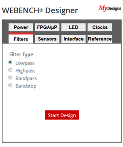
To access the WEBENCH Filter Designer, use http://ti.com/webenchfilters. In the box on the right side of View, select filter type (Lowpass, Highpass, Bandpass, or Bandstop) then click Start Design.

Specify Filter Requirements

Welcome to WEBENCH Filter Designer. The Filter Designer Requirements page is the first view you will see. See the figure below and read the text that follows.

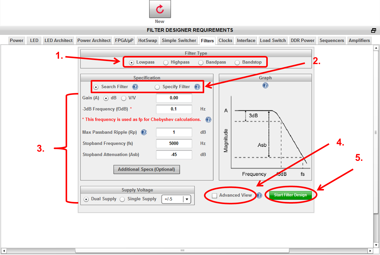
1.    Select desired filter response: Lowpass, Highpass, Bandpass, or Bandstop

2.    Adjust input style to match your design preference by selecting Search Filter or Specify Filter. Search Filter recommends filter approximations to meet your requirements. Specify Filter allows you to specify filter order and approximation type (e.g. 2^nd order, Butterworth filter).

3.    Enter desired frequency and gain parameters. Remember to enter the power supply voltage for your design at the bottom.

4.    You can start the filter design process using either Simple or Advanced mode. Simple mode, when the Advanced View is unchecked, creates a simplified view showing only the Solutions table and associated graphs.
Advanced mode, when the Advanced View is checked, shows the Solutions table and associated graphs, the WEBENCH Optimizer, and Advanced Charting windows.

5.     After selecting the mode, click Start Filter Design and proceed to the Filter Designer Visualizer page.

View and optimize filter response solutions with Filter Designer Visualizer

Filter Designer Visualizer (using Simple mode)

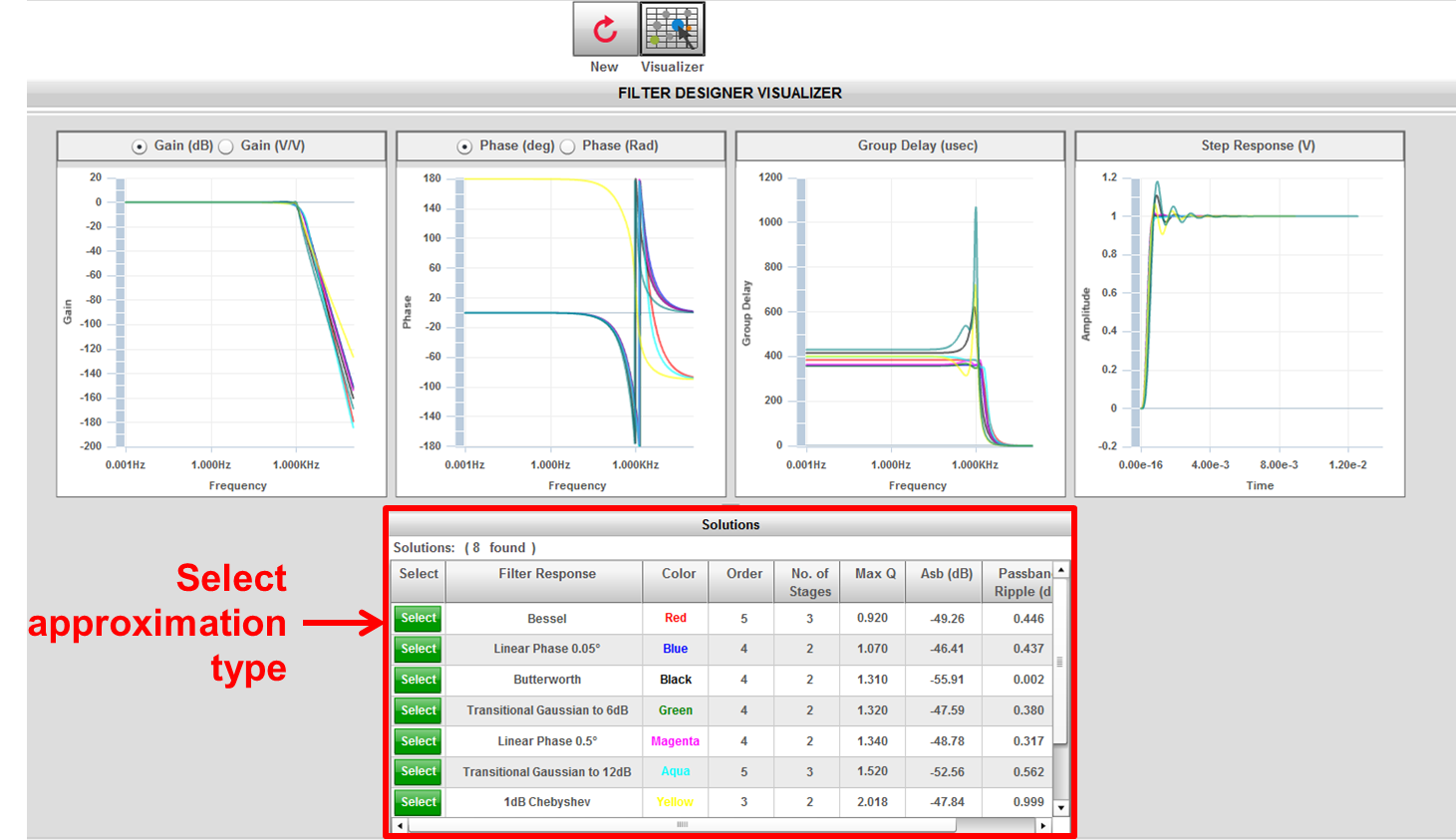
The top portion of this page shows the ideal gain, phase, group delay, and step response of the members in the solutions table below. If you hover your mouse over these curves, the approximation type, order, x-axis and y-axis values appear.

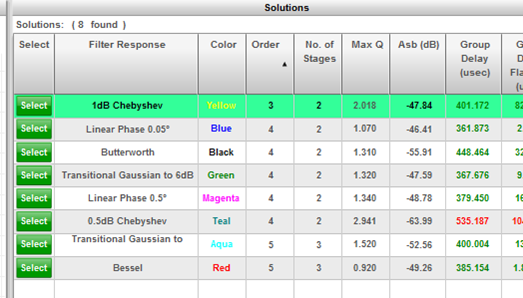
In the bottom portion of the page, a table with columns Select, Filter Response (or approximation), Color, Order, No. of stages, Max Q and Abs appear. Here is a description of these columns.

·         Select (green button) will take you with your chosen filter to the next page.

·         Filter Response has the available filter approximation types that comply with your inputs on the previous page.

·         Color relates to the graphs on the top of the page.

·         Order relates to the number of poles and zeros that a filter has in the design. For instance, for a 2^nd order filter:

The possible low pass and high pass filter orders are 1, 2, 3, 4, 5, 6, 7, 8, 9, and 10. The possible band pass and band stop filter orders are 2, 4, 6, 8, 10, 12, 14, 16, 18, and 20.

·         No. of stages describes the number of filter stages that your design will have.

·         Max Q defines the filter’s overall Q  or quality factor. This is equal to 1/(2*damping factor). If the maximum Q is less than 0.5, the system is overdamped. If  Q is equal to 0.5, the system is critically damped. If Q is higher than 0.5, the system is underdamped. For more detail about active filter’s quality factor refer to TI’s blog, Is your op amp filter ringing? Look at Q!

·         Abs is the stop-band attenuation at fs (stop-band frequency).

Once you find the filter that you want to build, click on the green Select button to proceed to the Schematic page. 

Filter Designer Visualizer (using advanced mode)

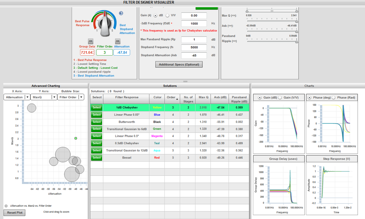
There are six sub-windows to help you zero in on your final filter design. Let’s start with the bottom three sub-windows.

The Solutions table has the same columns as simple mode. Please refer to that description of the Solutions table in the section above.

Charts also has the same ideal graphs as described for simple mode; gain, phase, group delay, and step response. Here in advanced mode, these graphs lets you zoom in on the curves to achieve more granularity. 

Advanced Charting allows you to see the solutions table’s active filters graphically. The x-axis, y-axis, and bubble size are represent the specification in the Solutions table columns. For instance, in the figure above the assignments are:

          x-axis – Abs 

          y-axis – Max Q

          bubble size – Filter order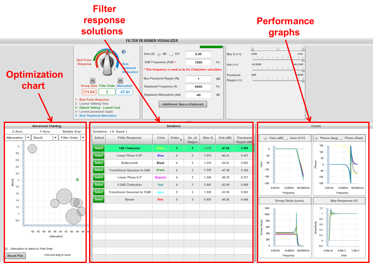     

Now we will discuss the top sub-windows.        

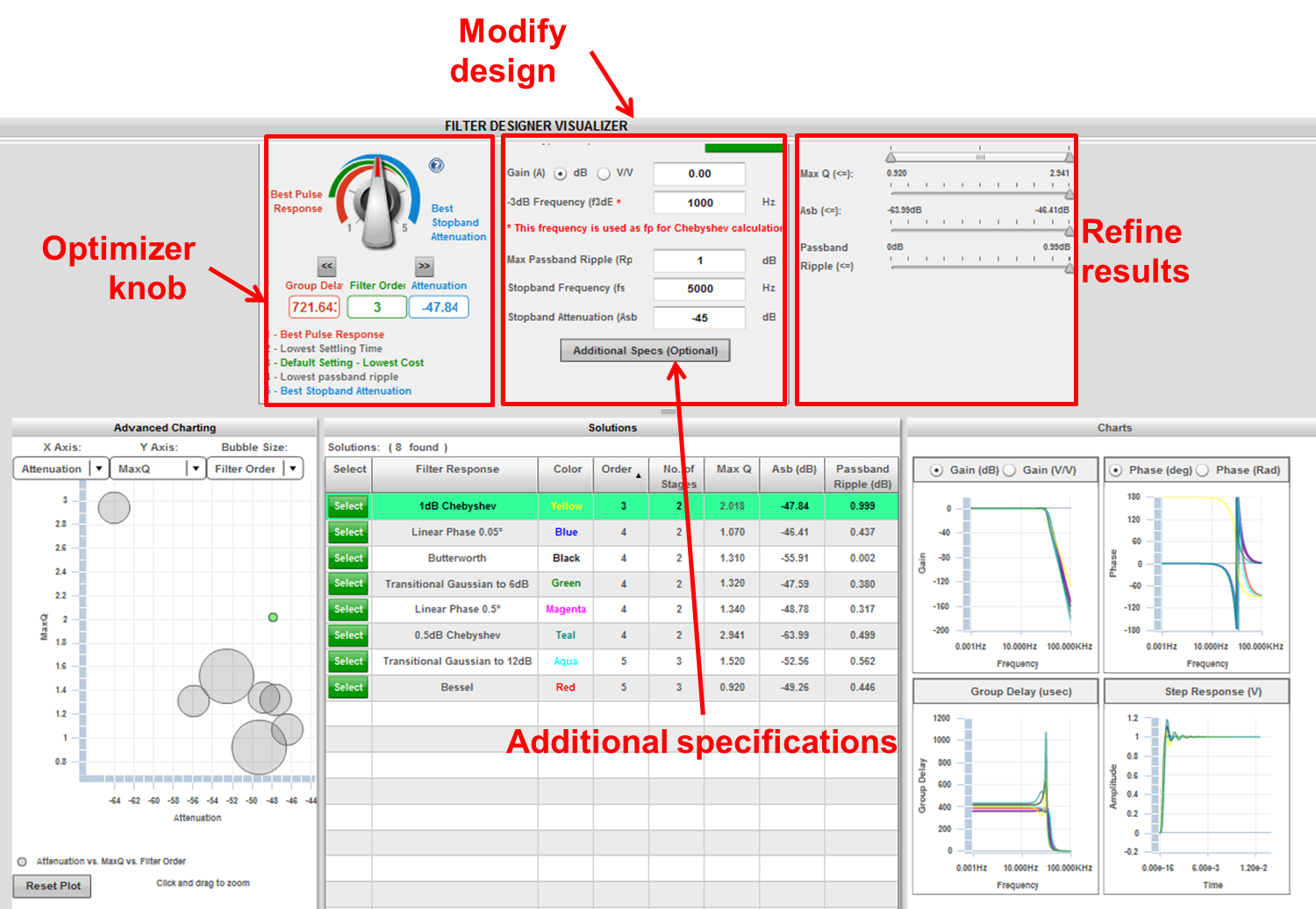
The Optimizer knob allows you to sort the filters in accordance to their characteristics. Notice that the order of the filters in the solutions table will re-sort with the best selection for your criteria on top. These characteristics are:

1.    Best Pulse Response favors designs with the lowest group delay, which generally provides best transient fidelity.

2.    Lowest Settling Time sorts designs to the top that result in the lowest settling time. In many cases, these also have the lowest group delay.

3.    Lowest Cost sorts the lowest cost amplifiers and the lowest order filters. This algorithm favors designs with a lower part count.

4.    Lowest Passband Ripple favors maximally flat pass-band responses

5.    Best Stopband Attenuation sorts designs to the top that provide the highest attenuation at the stop-band frequency.

Modify your original constraints by entering values in the Change Inputs fields and click Recalculate to immediately see the results of those modifications.

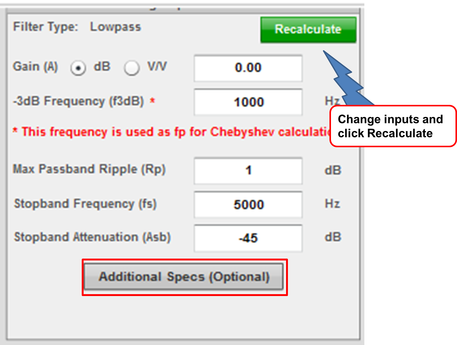
Additional Specs (Optional) button takes you to a page where you can control parameters and limits for group delay and step response. Your limits will determine whether the ideal filter calculations in the solutions table are within your specifications.

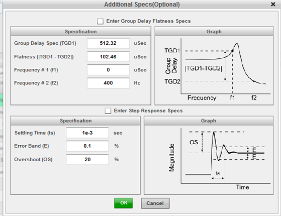
You will see in the Solutions table for Group Delay uses the font color to green to indicate pass and red for fail.

The Refine Results sliders provide another way to sort the filters. Click and move the sliders to narrow down the filter response choices.

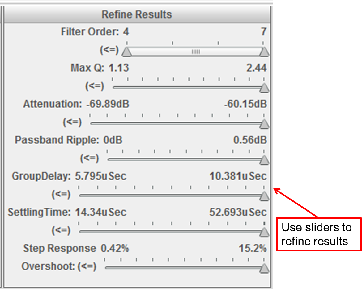
Once you find your filter, click on the green Select button to proceed to the design summary page showing the schematic.